Demo of a KDE plot beside timeseries set
%pylab inline
import pysd
import numpy as np
import pandas as pd
import seaborn
Populating the interactive namespace from numpy and matplotlib
Load the model using PySD
The model is a basic, 1-stock carbon bathtub model
model = pysd.read_vensim('../../models/Climate/Atmospheric_Bathtub.mdl')
print(model.doc)
                   Real Name                    Py Name Subscripts  Units  0                  Emissions                  emissions       None   None
1  Excess Atmospheric Carbon  excess_atmospheric_carbon       None   None
2                 FINAL TIME                 final_time       None  Month
3               INITIAL TIME               initial_time       None  Month
4            Natural Removal            natural_removal       None   None
5           Removal Constant           removal_constant       None   None
6                    SAVEPER                    saveper       None  Month
7                  TIME STEP                  time_step       None  Month
8                       Time                       time       None   None

       Limits       Type Subtype                                     Comment
0  (nan, nan)   Constant  Normal                                        None
1  (nan, nan)   Stateful   Integ                                        None
2  (nan, nan)   Constant  Normal          The final time for the simulation.
3  (nan, nan)   Constant  Normal        The initial time for the simulation.
4  (nan, nan)  Auxiliary  Normal                                        None
5  (nan, nan)   Constant  Normal                                        None
6  (0.0, nan)  Auxiliary  Normal  The frequency with which output is stored.
7  (0.0, nan)   Constant  Normal           The time step for the simulation.
8  (nan, nan)       None    None                  Current time of the model.
Generate a set of parameters to use as input
Here, drawing 100 constant values for the Emissions parameter from
an exponential distribution
n_runs = 100
runs = pd.DataFrame({'Emissions': np.random.exponential(scale=10000, size=n_runs)})
runs.head()
| Emissions | |
|---|---|
| 0 | 207.734860 |
| 1 | 7109.125870 |
| 2 | 4768.041210 |
| 3 | 2191.302602 |
| 4 | 16930.863016 |
Run the model with the various parameters
result = runs.apply(lambda p: model.run(params=dict(p))['Excess Atmospheric Carbon'],
                    axis=1).T
result.head()
| 0 | 1 | 2 | 3 | 4 | 5 | 6 | 7 | 8 | 9 | ... | 90 | 91 | 92 | 93 | 94 | 95 | 96 | 97 | 98 | 99 | |
|---|---|---|---|---|---|---|---|---|---|---|---|---|---|---|---|---|---|---|---|---|---|
| 0 | 0.000000 | 0.000000 | 0.000000 | 0.000000 | 0.000000 | 0.000000 | 0.000000 | 0.000000 | 0.000000 | 0.000000 | ... | 0.000000 | 0.000000 | 0.000000 | 0.000000 | 0.000000 | 0.000000 | 0.000000 | 0.000000 | 0.000000 | 0.000000 |
| 1 | 207.734860 | 7109.125870 | 4768.041210 | 2191.302602 | 16930.863016 | 14676.223891 | 2058.091604 | 9229.459073 | 1215.333008 | 22711.067942 | ... | 5438.319103 | 13029.384661 | 28268.791836 | 7543.867757 | 12566.422839 | 1565.757571 | 1029.656855 | 2802.757320 | 18335.083353 | 3311.616813 |
| 2 | 413.392371 | 14147.160482 | 9488.402008 | 4360.692179 | 33692.417401 | 29205.685543 | 4095.602292 | 18366.623556 | 2418.512686 | 45195.025205 | ... | 10822.255014 | 25928.475475 | 56254.895754 | 15012.296837 | 25007.181449 | 3115.857566 | 2049.017141 | 5577.487067 | 36486.815873 | 6590.117458 |
| 3 | 616.993307 | 21114.814748 | 14161.559198 | 6508.387860 | 50286.356243 | 43589.852579 | 6112.737873 | 27412.416393 | 3609.660567 | 67454.142895 | ... | 16152.351567 | 38698.575381 | 83961.138633 | 22406.041626 | 37323.532473 | 4650.456561 | 3058.183825 | 8324.469516 | 54457.031068 | 9835.833097 |
| 4 | 818.558233 | 28012.792471 | 18787.984817 | 8634.606583 | 66714.355696 | 57830.177944 | 8109.702098 | 36367.751302 | 4788.896970 | 89490.669408 | ... | 21429.147154 | 51340.974288 | 111390.319083 | 29725.848967 | 49516.719987 | 6169.709566 | 4057.258842 | 11043.982140 | 72247.544111 | 13049.091579 |
5 rows × 100 columns
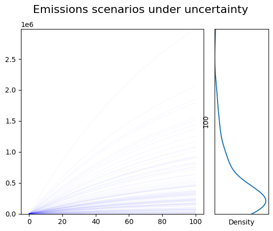
Draw a plot showing the results, and a marginal density plot
# left side should have all traces plotted
plt.subplot2grid((1,4), loc=(0,0), colspan=3)
[plt.plot(result.index, result[i], 'b', alpha=.02) for i in result.columns]
plt.ylim(0, max(result.iloc[-1]))

# right side has gaussian KDE on last timestamp
plt.subplot2grid((1,4), loc=(0,3))
seaborn.kdeplot(y=result.iloc[-1])
plt.ylim(0, max(result.iloc[-1]));
plt.yticks([])
plt.xticks([])

plt.suptitle('Emissions scenarios under uncertainty', fontsize=16);