Using SD models to understand the differences between population measures at varying levels of geographic disagregation

In this recipe, we will use data at a national level to infer parameters for a population aging model. We’ll then try two different ways of using this trained model to understand variation between the behavior of each of the states.

About this technique

Firstly, we’ll use the parameters fit at the national level to predict census data at the disaggregated level, and compare these predicted state-level outputs with the measured values. This gives us a sense for how different the populations of the states are from what we should expect given our understanding of the national picture.

Secondly, we’ll fit parameters to a model at each of the state levels actual measured census data, and then compare the differences in fit parameters to each other and to the national expectation. This is a helpful analysis if the parameter itself (and its inter-state variance) is what we find interesting.

%pylab inline
import pandas as pd
import pysd
import scipy.optimize
import geopandas as gpd

Populating the interactive namespace from numpy and matplotlib

Ingredients

Population data by age cohort

We start with data from the decennial census years 2000 and 2010, for the male population by state and county. We have aggregated the data into ten-year age cohorts (with the last cohort representing everyone over 80 years old). The data collection task is described here. In this analysis we will only use data at the state and national levels.

data = pd.read_csv('../../data/Census/Males by decade and county.csv', header=[0,1], index_col=[0,1])
data.head()

		2000									2010
		dec_1	dec_2	dec_3	dec_4	dec_5	dec_6	dec_7	dec_8	dec_9	dec_1	dec_2	dec_3	dec_4	dec_5	dec_6	dec_7	dec_8	dec_9
state	county
1	1	3375	3630	2461	3407	3283	2319	1637	825	284	3867	4384	3082	3598	4148	3390	2293	1353	454
	3	9323	10094	7600	9725	10379	8519	6675	4711	1822	11446	12006	9976	11042	12517	12368	10623	6307	2911
	5	2002	2198	2412	2465	2178	1699	1026	689	301	1673	1739	2260	2208	2233	1910	1490	739	324
	7	1546	1460	1680	1762	1624	1237	774	475	187	1471	1577	1798	2016	1928	1581	1140	579	211
	9	3741	3615	3393	3901	3773	3007	2227	1269	550	3741	4252	3312	3719	4129	3782	3052	1723	652

A model of an aging population

The model we’ll use to represent the population is a simple aging chain, with individuals aggregated into stocks by decade, to match the agregation we used for the above data. Each cohort is promoted with a timescale of 10 years, and there is some net inmigration, outmigration, and death subsumed into the loss flow associated with each cohort. This loss is controled by some yearly fraction that it will be our task to understand.

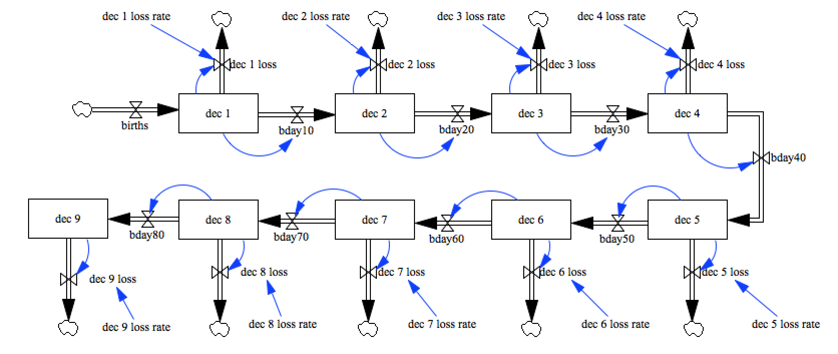
model = pysd.read_vensim('../../models/Aging_Chain/Aging_Chain.mdl')

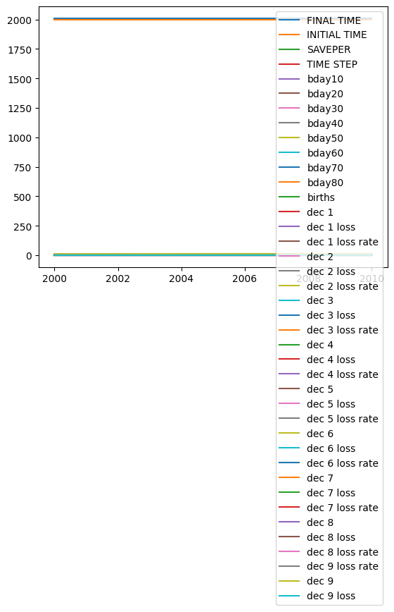
Our model is initialy parameterized with 10 individuals in each stock, no births, and a uniform loss rate of 5%. We’ll use data to set the initial conditions, and infer the loss rates. Estimating births is difficult, and so for this analysis, we’ll pay attention only to individuals who have been born before the year 2000.

model.run().plot();

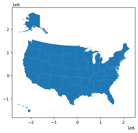
Geography Information

This information comes to us as a shape file .shp with its associated .dbf and .shx conspirator files. Lets check the plotting functionality:

state_geo = gpd.read_file('../../data/Census/US_State.shp')
state_geo.set_index('StateFIPSN', inplace=True)
state_geo.plot();
state_geo.head(2)

	CensusDiv	CensusReg	FIPS	FIPSNum	Notes	OBJECTID	StateFIPS	StateName	XCentroid	YCentroid	geometry
StateFIPSN
2	Pacific	West	02000	2000	None	1	02	Alaska	-1882092.15195	2310348.392810	(POLYGON ((-2247528.774479387 2237995.01157197...
53	Pacific	West	53000	53000	None	9	53	Washington	-1837353.15317	1340481.223852	(POLYGON ((-2124362.24278068 1480441.850674443...

Recipe Part A: Predict state-level values from national model fit

Step 1: Initialize the model using census data

We can aggregate the county level data to the national scale by summing across all geographies. This is relatively straightforward.

country = data.sum()
country

2000  dec_1    20332536
      dec_2    20909490
      dec_3    19485544
      dec_4    21638975
      dec_5    21016627
      dec_6    15115009
      dec_7     9536197
      dec_8     6946906
      dec_9     3060483
2010  dec_1    20703935
      dec_2    21878666
      dec_3    21645336
      dec_4    20033352
      dec_5    21597437
      dec_6    20451686
      dec_7    13926846
      dec_8     7424945
      dec_9     4083435
dtype: float64

If we run the model using national data from the year 2000 as starting conditions, we can see how the cohorts develop, given our arbitrary loss rate values:

model.run(return_timestamps=range(2000,2011),
          initial_condition=(2000, country['2000'])).plot();

Step 2: Fit the national level model to the remaining data

We’ve used half of our data (from the year 2000 census) to initialize our model. Now we’ll use an optimization routine to choose the loss rate parameters that best predict the census 2010 data. We’ll use the same basic operations described in the previous recipe: Fitting with Optimization.

To make this simple, we’ll write a function that takes a list of potential model parameters, and returns the model’s prediction in the year 2010

def exec_model(paramlist):
    params = dict(zip(['dec_%i_loss_rate'%i for i in range(1,10)], paramlist))
    output = model.run(initial_condition=(2000,country['2000']),
                       params=params, return_timestamps=2010)
    return output

Now we’ll define an error function that calls this executor and calculates a sum of squared errors value. Remember that because we don’t have birth information, we’ll only calculate error based upon age cohorts 2 through 9.

def error(paramlist):
    output = exec_model(paramlist)
    errors = output - country['2010']
    #don't tally errors in the first cohort, as we don't have info about births
    return sum(errors.values[0,1:]**2)

Now we can use the minimize function from scipy to find a vector of parameters which brings the 2010 predictions into alignment with the data.

res = scipy.optimize.minimize(error, x0=[.05]*9,
                              method='L-BFGS-B')
country_level_fit_params = dict(zip(['dec_%i_loss_rate'%i for i in range(1,10)], res['x']))
country_level_fit_params

{'dec_1_loss_rate': 0.021183432598200467,
 'dec_2_loss_rate': -0.052101419562612286,
 'dec_3_loss_rate': -0.0014091019293939956,
 'dec_4_loss_rate': 0.0088436979759478375,
 'dec_5_loss_rate': -0.0072046351581388701,
 'dec_6_loss_rate': -0.011046250905098235,
 'dec_7_loss_rate': 0.017228650364514753,
 'dec_8_loss_rate': 0.063195268137886118,
 'dec_9_loss_rate': 0.16077452197707129}

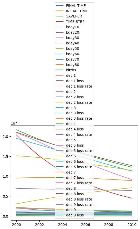
If we run the national model forwards with these parameters, we see generally good behavior, except for the 0-9yr demographic bracket, from whom we expect less self-control. (And because we don’t have births data.)

model.run(params=country_level_fit_params,
          return_timestamps=range(2000,2011),
          initial_condition=(2000, country['2000'])).plot();

Step 3: Make state-level predictions

If we want to look at the variances between the states and the national level, we can try making state-level predictions using state-specific initial conditions, but parameters fit at the national level.

states = data.sum(level=0)
states.head()

	2000									2010
	dec_1	dec_2	dec_3	dec_4	dec_5	dec_6	dec_7	dec_8	dec_9	dec_1	dec_2	dec_3	dec_4	dec_5	dec_6	dec_7	dec_8	dec_9
state
1	312841	329043	301076	315262	321447	246427	165327	109918	45131	312605	338568	321236	297502	321810	318358	229496	124070	56543
2	50687	53992	42537	51442	56047	35804	14974	7628	2325	53034	52278	58166	47753	51856	54170	29869	10392	4151
4	395110	384672	386486	391330	352471	257798	187193	144837	61148	463808	466275	455170	422447	418398	381076	300553	178849	89247
5	188589	201405	180801	187516	186931	149142	104621	72629	33050	201821	205074	196956	183761	192596	188081	143285	81138	38925
6	2669364	2588761	2556975	2812648	2495158	1692007	1002881	725610	331342	2573619	2780997	2849483	2595717	2655307	2336519	1489395	780576	456217

We can now generate a prediction by setting the model’s intitial conditions with state level data, and parameters fit in the national case. I’ve created a model_runner helper function to make the code easier to read, but this could be conducted in a single line if we so chose.

def model_runner(row):
    result = model.run(params=country_level_fit_params,
                       initial_condition=(2000,row['2000']),
                       return_timestamps=2010)
    return result.loc[2010]

state_predictions = states.apply(model_runner, axis=1)
state_predictions.head()

	dec_1	dec_2	dec_3	dec_4	dec_5	dec_6	dec_7	dec_8	dec_9
state
1	93117.371881	341167.213342	337071.875334	304311.201330	325833.277920	316445.464900	223627.149408	121168.476612	65739.525962
2	15087.025659	55697.612356	52613.730625	47359.482364	53391.883377	50862.893499	31762.129879	14297.875847	6133.949764
4	117604.805785	411745.021973	413024.709292	377589.072369	386843.833461	354697.832262	246306.408711	138031.543558	79499.152922
5	56133.665931	207553.388634	204417.938099	183004.303895	192875.524445	187772.888790	135135.556656	75209.777699	42570.643627
6	794538.317812	2775504.193632	2765302.000982	2586476.416275	2709538.756509	2450307.128284	1595568.711162	818892.701581	439955.979351

Step 4: Compare model predictions with measured data

Comparing the state level predictions with the actual data, we can see where our model most under or overpredicts population for each region/cohort combination.

diff = state_predictions-states['2010']
diff.head()

	dec_1	dec_2	dec_3	dec_4	dec_5	dec_6	dec_7	dec_8	dec_9
state
1	-219487.628119	2599.213342	15835.875334	6809.201330	4023.277920	-1912.535100	-5868.850592	-2901.523388	9196.525962
2	-37946.974341	3419.612356	-5552.269375	-393.517636	1535.883377	-3307.106501	1893.129879	3905.875847	1982.949764
4	-346203.194215	-54529.978027	-42145.290708	-44857.927631	-31554.166539	-26378.167738	-54246.591289	-40817.456442	-9747.847078
5	-145687.334069	2479.388634	7461.938099	-756.696105	279.524445	-308.111210	-8149.443344	-5928.222301	3645.643627
6	-1779080.682188	-5492.806368	-84180.999018	-9240.583725	54231.756509	113788.128284	106173.711162	38316.701581	-16261.020649

This is a little easier to understand if we weight it by the actual measured population:

diff_percent = (state_predictions-states['2010'])/states['2010']
diff_percent.head()

	dec_1	dec_2	dec_3	dec_4	dec_5	dec_6	dec_7	dec_8	dec_9
state
1	-0.702124	0.007677	0.049297	0.022888	0.012502	-0.006007	-0.025573	-0.023386	0.162647
2	-0.715522	0.065412	-0.095456	-0.008241	0.029618	-0.061051	0.063381	0.375854	0.477704
4	-0.746436	-0.116948	-0.092592	-0.106186	-0.075417	-0.069220	-0.180489	-0.228223	-0.109223
5	-0.721864	0.012090	0.037886	-0.004118	0.001451	-0.001638	-0.056876	-0.073063	0.093658
6	-0.691276	-0.001975	-0.029543	-0.003560	0.020424	0.048700	0.071286	0.049088	-0.035643

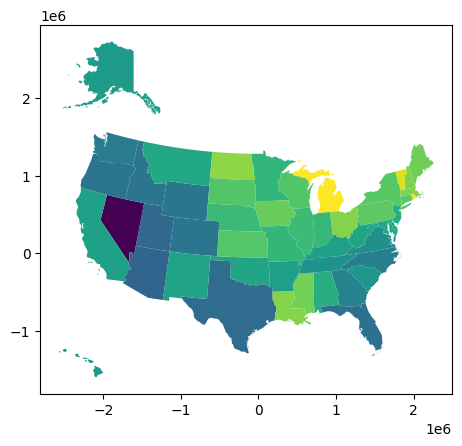
Step 5: Merge with geo data to plot

I’m using geopandas to manage the shapefiles, and it has its own plotting functionality. Unfortunately, it is not a particularly well defined functionality.

geo_diff = state_geo.join(diff_percent)
geo_diff.plot(column='dec_4')
geo_diff.head()

	CensusDiv	CensusReg	FIPS	FIPSNum	Notes	OBJECTID	StateFIPS	StateName	XCentroid	YCentroid	geometry	dec_1	dec_2	dec_3	dec_4	dec_5	dec_6	dec_7	dec_8	dec_9
StateFIPSN
2	Pacific	West	02000	2000	None	1	02	Alaska	-1882092.151950	2310348.392810	(POLYGON ((-2247528.774479387 2237995.01157197...	-0.715522	0.065412	-0.095456	-0.008241	0.029618	-0.061051	0.063381	0.375854	0.477704
53	Pacific	West	53000	53000	None	9	53	Washington	-1837353.153170	1340481.223852	(POLYGON ((-2124362.24278068 1480441.850674443...	-0.718560	-0.006548	-0.058893	-0.069401	-0.018494	-0.031807	-0.047478	0.013500	-0.030573
23	New England	Northeast	23000	23000	None	10	23	Maine	2068849.532637	1172786.748295	(POLYGON ((1951177.135094963 1127914.539498126...	-0.682708	0.073037	0.147467	0.085983	-0.023217	-0.055249	-0.076098	-0.034226	-0.009394
27	West North Central	Midwest	27000	27000	None	11	27	Minnesota	131047.575089	982130.006959	POLYGON ((-91052.16805501282 1282100.079225723...	-0.711546	0.062669	0.034611	0.032717	0.020127	-0.019902	0.043175	0.022524	-0.060437
26	East North Central	Midwest	26000	26000	None	18	26	Michigan	842567.889298	809437.260865	(POLYGON ((764918.7306621727 786184.882347865,...	-0.657411	0.082088	0.197840	0.176409	0.088111	0.032552	0.050903	0.075986	0.011505

Recipe Part B: fit state-by-state models

Now lets try optimizing the model’s parameters specifically to each state, and comparing with the national picture.

Step 1: Write the optimization functions to account for the state

We’ll start as before with functions that run the model and compute the error (this time with a parameter for the information about the state in question) and add a function to optimize and return the best fit parameters for each state.

def exec_model(paramlist, state):
    params = dict(zip(['dec_%i_loss_rate'%i for i in range(1,10)], paramlist))
    output = model.run(initial_condition=(2000,state['2000']),
                       params=params, return_timestamps=2010).loc[2010]
    return output

def error(paramlist, state):
    output = exec_model(paramlist, state)
    errors = output - state['2010']
    #don't tally errors in the first cohort, as we don't have info about births
    sse = sum(errors.values[1:]**2)
    return sse

Step 2: Apply optimization to each state

We can wrap the optimizer in a function that takes census information about each state and returns an optimized set of parameters for that state. If we apply it to the states dataframe, we can get out a similar dataframe that includes optimized parameters.

%%capture
def optimize_params(row):
    res = scipy.optimize.minimize(lambda x: error(x, row),
                                  x0=[.05]*9,
                                  method='L-BFGS-B');
    return pd.Series(index=['dec_%i_loss_rate'%i for i in range(1,10)], data=res['x'])

state_fit_params = states.apply(optimize_params, axis=1)
state_fit_params.head()

	dec_1_loss_rate	dec_2_loss_rate	dec_3_loss_rate	dec_4_loss_rate	dec_5_loss_rate	dec_6_loss_rate	dec_7_loss_rate	dec_8_loss_rate	dec_9_loss_rate
state
1	0.021448	-0.051229	0.005996	0.009159	-0.006314	-0.012721	0.013077	0.061467	0.199157
2	0.024790	-0.045179	-0.021897	0.015292	-0.003120	-0.023723	0.039461	0.137920	0.200484
4	0.015650	-0.066072	-0.009319	-0.003544	-0.012930	-0.018060	-0.013545	0.033047	0.168508
5	0.022108	-0.050841	0.003923	0.005605	-0.006411	-0.011430	0.006571	0.054650	0.191023
6	0.020025	-0.052080	-0.006135	0.010332	-0.004042	-0.004572	0.025891	0.065019	0.148008

Step 3: Merge with geographic data

As we’re looking at model parameters which themselves are multiplied by populations to generate actual flows of people, we can look at the difference between parameters directly without needing to normalize.

geo_diff = state_geo.join(state_fit_params)
geo_diff.plot(column='dec_4_loss_rate')
geo_diff.head(3)

	CensusDiv	CensusReg	FIPS	FIPSNum	Notes	OBJECTID	StateFIPS	StateName	XCentroid	YCentroid	geometry	dec_1_loss_rate	dec_2_loss_rate	dec_3_loss_rate	dec_4_loss_rate	dec_5_loss_rate	dec_6_loss_rate	dec_7_loss_rate	dec_8_loss_rate	dec_9_loss_rate
StateFIPSN
2	Pacific	West	02000	2000	None	1	02	Alaska	-1882092.151950	2310348.392810	(POLYGON ((-2247528.774479387 2237995.01157197...	0.024790	-0.045179	-0.021897	0.015292	-0.003120	-0.023723	0.039461	0.137920	0.200484
53	Pacific	West	53000	53000	None	9	53	Washington	-1837353.153170	1340481.223852	(POLYGON ((-2124362.24278068 1480441.850674443...	0.021844	-0.053040	-0.010785	0.001392	-0.006107	-0.015620	0.010874	0.072777	0.150871
23	New England	Northeast	23000	23000	None	10	23	Maine	2068849.532637	1172786.748295	(POLYGON ((1951177.135094963 1127914.539498126...	0.025517	-0.044513	0.016994	0.013372	-0.014052	-0.017986	0.007721	0.065287	0.161693