Exogenous model input from a file

In this notebook we’ll demonstrate using an external data source to feed values into a model. We’ll use the carbon emissions dataset, and feed total emissions into a stock of excess atmospheric carbon:

We’ll begin as usual by importing PySD and the machinery we need in order to deal with data manipulation and plotting.

%pylab inline
import pysd
import pandas as pd

Populating the interactive namespace from numpy and matplotlib

We use Pandas library to import emissions data from a .csv file. In this command, we both rename the columns of the dataset, and set the index to the ‘Year’ column.

emissions = pd.read_csv('../../data/Climate/global_emissions.csv',
                        skiprows=2, index_col='Year',
                        names=['Year', 'Total Emissions',
                               'Gas Emissions', 'Liquid Emissions',
                               'Solid Emissions', 'Cement Emissions',
                               'Flare Emissions', 'Per Capita Emissions'])
emissions.head()

	Total Emissions	Gas Emissions	Liquid Emissions	Solid Emissions	Cement Emissions	Flare Emissions	Per Capita Emissions
Year
1751	3	0	0	3	0	0	NaN
1752	3	0	0	3	0	0	NaN
1753	3	0	0	3	0	0	NaN
1754	3	0	0	3	0	0	NaN
1755	3	0	0	3	0	0	NaN

model = pysd.read_vensim('../../models/Climate/Atmospheric_Bathtub.mdl')

In our vensim model file, the value of the inflow to the carbon bathtub, the Emissions parameter, is set to zero. We want to instead have this track our exogenous data.

Emissions=
    0

Excess Atmospheric Carbon= INTEG (
    Emissions - Natural Removal,
    0)

Natural Removal=
    Excess Atmospheric Carbon * Removal Constant

Removal Constant=
    0.01

Aligning the model time bounds with that of the dataset

Before we can substitute in our exogenous data, however, we need to ensure that the model will execute over the proper timeseries. The initial and final times of the simulation are specified in the model file as:

print('initial:', model.components.initial_time())
print('final:', model.components.final_time())

initial: 0
final: 100

However, the time frame of the dataset runs:

print('initial:', emissions.index[0])
print('final:', emissions.index[-1])

initial: 1751
final: 2011

In order to run the model over a time series equal to that of the data set, we need to specify the appropriate initial conditions, and ask the run function to return to us timestamps equal to that of our dataset:

res = model.run(initial_condition=(emissions.index[0],
                                   {'Excess Atmospheric Carbon': 0}),
                return_timestamps=emissions.index.values,
                return_columns=['Emissions', 'Excess Atmospheric Carbon'])
res.head()

	Emissions	Excess Atmospheric Carbon
1751	0	0.0
1752	0	0.0
1753	0	0.0
1754	0	0.0
1755	0	0.0

Pass in our timeseries data

In place of the constant value of emissions, we want to substitute our dataset. We can do this in a very straightforward way by passing the Pandas Series corresponding to the dataset in a dictionary to the params argument of the run function.

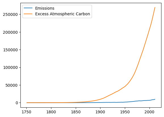
res = model.run(initial_condition=(emissions.index[0],
                                   {'Excess Atmospheric Carbon': 0}),
                return_timestamps=emissions.index.values,
                return_columns=['Emissions', 'Excess Atmospheric Carbon'],
                params={'Emissions': emissions['Total Emissions']})

res.plot();